Temporal Inertia Law: Why Temporal Space Cannot Change Instantaneously
1. Introduction
Temporal Space is not a collection of isolated timestamps. It behaves as a continuous field. Every temporal state is connected to neighboring states through measurable transition probabilities. This implies that Temporal Space cannot instantly reorganize itself. Instead, every structural change requires time.
2. Transition Matrix
The transition probability matrix reveals an unexpected property.
For all density states:
P(T→T)=0.73–0.92
Transitions to neighboring densities:
P(T→T±1)=0.07–0.14
Transitions larger than one density level:
P(T→T±2)<0.02
These probabilities form an almost perfectly tridiagonal matrix. Large structural jumps are practically absent.
4. Autocorrelation
Spatial memory confirms the same phenomenon.
Autocorrelation values:
- Lag 1: 0.981
- Lag 5: 0.940
- Lag 30: 0.815
- Lag 60: 0.721
- Lag 1440: ≈0
This means that neighboring temporal coordinates remain highly correlated. Only after approximately one day does the system completely lose memory of its previous configuration.
5. Practical Consequences
Temporal inertia produces predictable behavior. When density begins increasing: it usually continues increasing. When density begins decreasing: it usually continues decreasing. The field rarely changes direction abruptly. This significantly improves the stability of timing-based forecasting.
6. Difference from Price
Price frequently appears chaotic. Temporal density does not. Price reacts. Temporal Space evolves. Price may jump. Temporal density flows. This distinction explains why timing structures remain statistically reproducible while price trajectories remain highly variable.
Conclusion
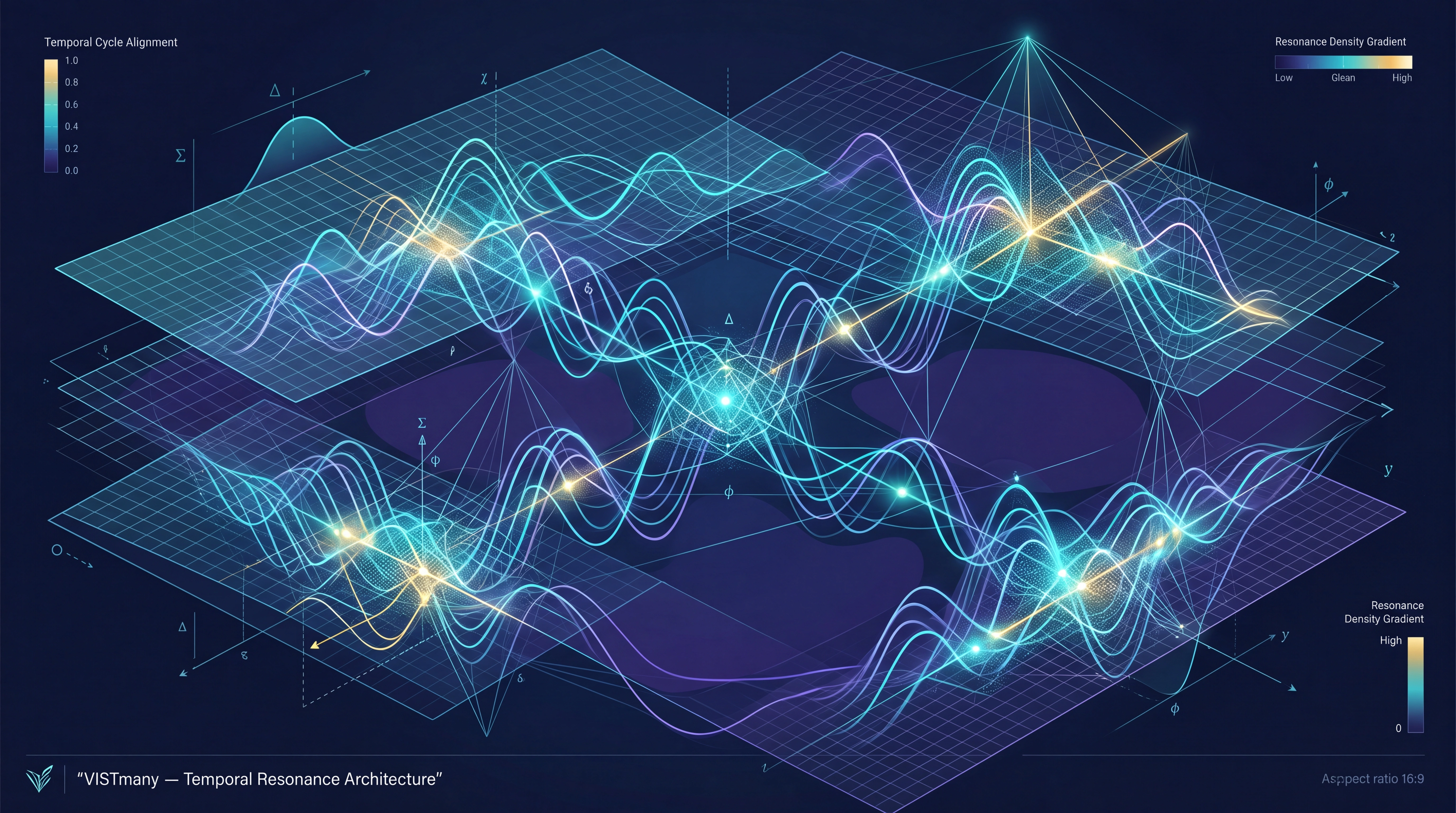
Temporal Space demonstrates measurable inertia. Its evolution follows continuous transition dynamics rather than random jumps. The Temporal Inertia Law provides a mathematical explanation for the remarkable stability observed in VISTmany timing structures across different historical periods and financial instruments.
The concept is directly connected to Temporal Space, Temporal Density, and Temporal Spectrum, all defined in the VISTmany Terminology page.